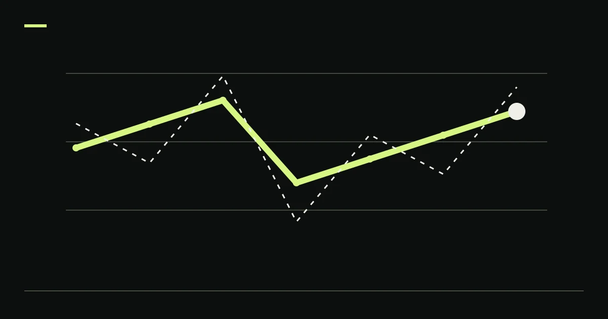
A crypto Monte Carlo trade-sequence test generates alternative paths under a declared sampling model. Shuffling keeps the same trades and changes their order; sampling with replacement can repeat or omit trades. These answer different questions. Neither creates evidence of market events missing from the original sample, and neither can repair biased source trades or establish a reliable future loss boundary by itself.
Before reading a fan of simulated equity curves, ask what was randomized. The curve count is less informative than the rule that created each curve.
Four trades are enough to separate path from profit
Use this original hypothetical dataset: four completed trades with fixed net dollar outcomes of +$100, −$100, +$100 and −$100. Start with $1,000. Assume no simultaneous positions, no additional costs, no cash flows and no account rule that changes or stops trades after a loss. These are constructed arithmetic inputs, not observed KLINEO trades.
Every ordering contains the same two gains and two losses, so every path ends at $1,000. The path between those endpoints can differ substantially.
| Unique order of outcomes | Equity after each trade, starting after the initial $1,000 | Maximum observed drawdown |
|---|---|---|
| +100, +100, −100, −100 | $1,100; $1,200; $1,100; $1,000 | 16.67%, rounded |
| +100, −100, +100, −100 | $1,100; $1,000; $1,100; $1,000 | 9.09%, rounded |
| +100, −100, −100, +100 | $1,100; $1,000; $900; $1,000 | 18.18%, rounded |
| −100, +100, +100, −100 | $900; $1,000; $1,100; $1,000 | 10.00% |
| −100, +100, −100, +100 | $900; $1,000; $900; $1,000 | 10.00% |
| −100, −100, +100, +100 | $900; $800; $900; $1,000 | 20.00% |
There are six unique value sequences because 4! / (2! × 2!) = 6. We enumerated all six rather than estimating them through random sampling. Maximum drawdown is computed relative to each path's running peak, including the initial balance. The drawdown and recovery worksheet defines that calculation.
The range from 9.09% to 20% describes these six constructed sequences. It is not a forecast interval for a real account. A fifth trade with a larger loss is absent from the sample and therefore absent from this permutation exercise.
A shuffle preserves more than its chart suggests
A permutation changes order without changing the sample's contents. In the fixed-dollar example, total P&L, win count and average outcome stay unchanged. The simulated exercise varies path-dependent quantities such as drawdown and consecutive losses.
NumPy's permutation interface makes this operation explicit: an array is copied with its elements randomly reordered. That is a software operation, not a statistical guarantee that the reordered trades are plausible future observations. NumPy permutation documentation
The same terminal-value invariance applies to a fixed list of simple percentage returns compounded without path-dependent constraints: multiplication of the factors does not depend on order. If an implementation reports different endpoints after only reordering that identical list, inspect sizing, rounding, omitted trades, stopping rules or an accounting error.
A real risk rule can legitimately make endpoints differ. If trading stops when equity breaches a threshold, some later trades no longer occur. The simulated object then includes that stopping rule. State it clearly and recompute the path as a process rather than adding all original trades regardless of account state.
Sampling with replacement creates a different experiment
Now draw four outcomes independently from the invented sample, allowing replacement. Each draw has a 50% chance of +$100 and a 50% chance of −$100 because the source sample contains equal counts. A path can contain four wins and end at $1,400, or four losses and end at $600.
Under these explicit artificial assumptions, each of those extreme sequences has probability (1/2)^4 = 6.25%. That is a property of this chosen resampling model. It does not estimate the probability of a $400 gain or loss in live crypto trading.
NumPy's choice interface distinguishes sampling with and without replacement, including optional sampling probabilities. The default replacement behavior permits an input value to be selected more than once. Record the actual options instead of using “Monte Carlo” as a complete method description. NumPy choice documentation
Changing the probabilities is another model assumption. If adverse outcomes receive extra weight for a stress case, label that scenario and show the chosen weights. Do not present the resulting percentile as an estimate recovered from unchanged historical frequencies.
Preserve the dependencies the question needs
Independent trade draws remove the original adjacency of losses. A strategy exposed to a persistent market regime may experience several related unfavorable outcomes together. Randomizing individual trades can break that clustering and alter the loss paths being studied.
Block resampling preserves the order of observations inside selected blocks. It still changes relationships across block boundaries and requires a justified block definition and length. Longer blocks retain more local structure while providing fewer distinct recombinations from a short sample. There is no universal block length that validates every strategy.
Politis and Romano's original stationary-bootstrap research introduces resampling with random-length blocks for weakly dependent stationary observations. Its statistical setting carries assumptions that must be examined before applying the method to trading data. It does not imply that any historical crypto return series is stationary or that block resampling recovers an unobserved future regime. The Stationary Bootstrap
Preserve simultaneous portfolio exposure as well. Independently resampling two coin strategies can remove a shared market shock if they actually traded during the same event. For a portfolio question, a synchronized return vector or another explicit joint model may be more appropriate than unrelated trade lists.
Keep the sampling unit compatible with the metric
Completed trades have unequal durations. Shuffling their outcomes creates an event-order path, not automatically a calendar-day equity series. The exercise cannot supply elapsed recovery time or daily risk ratios without a declared timing model.
A Sharpe or Sortino calculation needs a compatible periodic return series. Do not annualize a trade-order sequence as though every trade took exactly one day unless that is an explicit and defensible assumption.
Costs and sizing also belong in the sampling unit. Resampling gross P&L and attaching a single average fee can obscure the relationship between trade size, adverse execution and market conditions. If costs change with volatility or liquidity, keep the relevant observations together or specify how the synthetic model changes them.
Distinguish resampling returns from resampling prices. Shuffling candles can disrupt indicator history, gaps, session structure and the relationship between entries and subsequent prices. It evaluates a different synthetic-market construction, which needs its own rationale and execution model.
Percentiles describe the specified model
A statement such as “95th-percentile drawdown” needs its sample length, sampling unit, replacement rule, dependence treatment, path length, sizing rule and percentile convention. It also needs the count of simulated paths and the random generator settings used for reproducibility.
More paths can reduce simulation noise within the same model. They do not expand the historical sample or validate the model's assumptions. A million resamples of four trades still depend on four observed outcomes and the chosen mechanism for recombining them.
If an actual risk threshold matters, report how many simulated paths cross it and what actions the modeled account takes afterward. Define “ruin” explicitly: zero equity, a margin liquidation event, a minimum operating balance and a chosen drawdown limit are different events.
Test sensitivity to the sampling rule and preserve unfavorable scenarios. Selecting the method that produces the smallest tail loss is another research choice. Its selection history belongs beside the output, much like the frozen schedule in walk-forward testing.
Decide what the exercise earns
Use an enumerated or simulated sequence exercise to identify path sensitivity under stated assumptions. If plausible clustering or a different block convention changes the result materially, retain that dependency in the conclusion. Do not translate a percentile into a guaranteed loss allowance.
Before resampling, inspect the original trades for causal signals, realistic costs and ambiguous fills using the backtest evidence review. Then compare the frozen logic in a supported paper validation, retaining the distinction between signal behavior and simulated execution quality.
Method and limits
This article was prepared with AI assistance. The four-trade dataset, six unique permutations and replacement example are original hypothetical illustrations. All sequences, running peaks, endpoints and probabilities were independently enumerated or calculated. No market-data bootstrap, KLINEO strategy simulation, prospective percentile or real account risk-of-ruin estimate was performed. These examples explain model boundaries and leave the risks of trading unresolved.