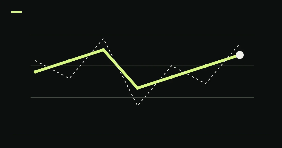
Crypto Sharpe and Sortino ratios summarize periodic returns using different measures of variation. A historical Sharpe ratio divides average excess return by the standard deviation of those excess returns. A Sortino ratio compares average return with a declared target and divides by downside deviation. Neither has a useful interpretation until the return interval, benchmark or target, costs and denominator convention are stated.
Two dashboards can display different ratios for the same six returns without either making a simple arithmetic mistake. The disagreement may be the definition they applied.
Begin with the series, not the headline
Request the periodic portfolio return series used in the calculation. Identify its currency, timestamps, treatment of open positions, external cash flows and all included costs. Trade P&L divided by order notional is different from daily account return. Mixing the two can make a comparison meaningless.
The excess return for each period is the portfolio return minus the chosen same-period benchmark return. A conventional cash-benchmark Sharpe calculation needs an appropriate benchmark series and interval. Assuming zero is a modeling choice that must be stated; an exchange stablecoin balance is not automatically equivalent to a risk-free investment.
William Sharpe's original discussion distinguishes historical differential returns from prospective values and emphasizes the time dependence of the ratio. It also explains that conventional time scaling becomes more complicated with compounding and serial correlation. Sharpe's 1994 article
Preserve that distinction when reading a backtest. A historical statistic describes the selected series. It is not automatically an unbiased forecast of the same statistic in live trading.
Recompute one six-period example
The following returns are an original hypothetical dataset. Each row is one equal-length period, with all modeled costs already deducted and no external cash flows. Use a zero benchmark and zero Sortino target solely to make the arithmetic transparent. The values are not historical crypto returns or KLINEO performance.
| Period | Net simple return | Deviation from sample mean | Squared downside shortfall versus zero, in percentage points squared |
|---|---|---|---|
| 1 | −2% | −3 percentage points | 4 |
| 2 | +1% | 0 percentage points | 0 |
| 3 | +3% | +2 percentage points | 0 |
| 4 | −1% | −2 percentage points | 1 |
| 5 | +2% | +1 percentage point | 0 |
| 6 | +3% | +2 percentage points | 0 |
The arithmetic mean is (-2 + 1 + 3 - 1 + 2 + 3) / 6 = 1% per period. For the sample standard deviation used here, divide the sum of squared mean deviations by 6 − 1. Those squares sum to 9 + 0 + 4 + 4 + 1 + 4 = 22, giving sqrt(22 / 5) = 2.0976 percentage points, rounded.
The resulting unannualized sample Sharpe ratio is 1 / 2.0976, approximately 0.4767. This calculation uses the sample standard-deviation convention. A calculation using a different denominator needs its own label and will produce a different value for such a small sample.
Keep units consistent. Dividing 0.01 by 0.020976 gives the same ratio as dividing 1 by 2.0976. Dividing 1 by 0.020976 mixes percentages with decimals and creates a result one hundred times too large.
The Sortino denominator must identify every included period
For this article's empirical downside deviation, take each return's shortfall below the zero target, square it, sum across the sample, divide by all six periods and take the square root. Returns above target contribute zero to the sum. The result is sqrt((4 + 1) / 6) = 0.9129 percentage points, rounded.
The unannualized Sortino ratio under that convention is 1 / 0.9129, approximately 1.0954. Its larger value than the example Sharpe ratio follows from the chosen downside denominator. It is not evidence that the same portfolio suddenly became safer.
If a report instead divides by only the two below-target observations, its downside measure becomes sqrt(5 / 2) = 1.5811 percentage points and its corresponding ratio is approximately 0.6325. That conditional calculation answers a different denominator question. Displaying both as interchangeable “Sortino ratios” conceals the convention.
CFA Institute's Sortino discussion notes variations in downside-deviation calculation and the importance of a consistent minimum acceptable return when comparing portfolios. It also discusses limitations for asymmetric return distributions. Use the definition actually implemented by the report. CFA Institute on the Sortino ratio
A zero downside deviation needs explicit treatment. If none of the observed periods falls below target, the sample does not provide an ordinary finite ratio through division by zero. Printing an impressive arbitrary ceiling hides the missing denominator evidence. Six favorable observations also cannot establish that losses are impossible.
A different target changes the question
Keep the six invented returns and raise the per-period Sortino target to 0.5%. The mean return above target becomes 0.5 percentage points. Only the −2% and −1% observations fall below this chosen target, with shortfalls of 2.5 and 1.5 percentage points.
Using the same full-sample denominator, downside deviation is sqrt((2.5^2 + 1.5^2) / 6), approximately 1.1902 percentage points. The resulting ratio is approximately 0.4201. The portfolio observations did not change. The target used to evaluate them did.
A target should be economically meaningful for the stated purpose, and its time unit must match the return series. Copying an annual percentage directly into a daily calculation produces a different hurdle. If converting targets across intervals, disclose the conversion method rather than assuming an arithmetic division and a compounded conversion are identical.
For comparisons, retain the same target, sample interval, cost basis and calculation convention. Even then, the two portfolios can have different liquidity, concentration and exposure that a single ratio does not describe.
Annualization requires more than a calendar multiplier
The familiar square-root-of-periods scaling rests on assumptions about return aggregation and serial dependence. Crypto trading can be observed on calendar days, trading-event intervals or other schedules. State which one the series uses and how many periods its annualization assumes.
Do not annualize this six-period demonstration into an implied investable result. Its purpose is to expose arithmetic conventions, and its short, invented sample contains no evidence about annual behavior. More decimal places or a larger annualization multiplier do not add observations.
Look for zero-return periods too. An account that sits in cash between trades still has a periodic return history. Removing inactive days changes both the average and the variability being measured. A trade-only series and a full-calendar account series need different descriptions.
When returns cluster, simple reordering can destroy the dependence relevant to risk. The Monte Carlo trade-sequence guide explains why simulated path counts do not replace a justified return model.
A high ratio can survive several different defects
Stale valuation can make returns appear smooth. Omitted costs can raise the numerator. Repeated parameter searches can select an unusually favorable ratio. Each issue needs its own evidence; choosing Sortino instead of Sharpe does not repair the underlying series.
Review the research trial ledger before interpreting a winning ratio selected from many alternatives. Selection-adjusted methods require information about those alternatives and their dependence. A final screenshot cannot supply it.
Also inspect the maximum drawdown and recovery path. Periodic mean and deviation do not identify the timing of the deepest loss, the duration of an unrecovered episode or whether capital was added during the decline.
The trade-expectancy worksheet provides a complementary reconciliation at the completed-position level. If trade totals and periodic portfolio returns do not reconcile after holdings and flows are accounted for, resolve that discrepancy before comparing ratios.
A compact evidence request
Ask the author to supply the exact return column, same-period benchmark or target column, observation count, missing-period policy, standard-deviation convention, downside denominator and annualization rule. Recompute one period and then the unannualized ratio. Finally reconcile the underlying series with marked equity and costs.
For KLINEO's published historical material, consult the stated input and reporting boundaries in the backtest methodology. Do not infer that every metric in a separate report uses this article's illustrative conventions.
Method and limits
This article was prepared with AI assistance using linked primary materials and an original six-period dataset. Means, sample deviation, both downside denominators and the alternate-target calculation were independently recomputed. No live portfolio, historical KLINEO ratio or statistical significance test was analyzed. Ratios assist comparison within a defined measurement model and do not establish future profitability or remove the risks of trading.